During the past 7 business days I took part in a training about SIMATIC IT XHQ 4.0 software.
I participated in the Basic (21-22 Jan) and Advanced (25-29 Jan) training.

This training was given by the engineer Fabio Terasaka who’s a team lead at Chemtech having over 3 years of experience using and deploying XHQ in Brazil and internationally.

I decided to write this post so that people can get an overview of XHQ from a consultant/developer perspective.

I’m also excited about the endless possibilities XHQ has to offer when it comes to optimizing and applying intelligence to an enterprise.

What is XHQ?
For those who don’t know or who have never heard of XHQ, here goes a succinct description of it extracted from its official site:

SIMATIC IT XHQ Operations Intelligence product line aggregates, relates and presents operational and business data in real-time to improve enterprise performance. Through SIMATIC IT XHQ, you have a single coherent view of information, enabling a variety of solutions in real-time performance management and decision support. ^[1]

XQH extracts data from a variety of systems - as the production (PIMS), laboratory (LIMS) and plant-floor systems. XHQ unifies all the operational and management data in a single view, in real time, allowing you to take a snapshot, minute to minute or second to second, of all the enterprise.

XHQ can be integrated in the intranet or a website for operations management, integrating production data such as the use of raw material and equipment, stocks, as well as data related to the product (temperature, pressure, electrical current), quality and maintenance.

XHQ implements the concepts of Operational Dashboard and Management ^[2] by Key Performance Indicators (KPIs) ^[3].

XHQ is used in energy, petrochemical, and manufacturing industries to aggregate, draw relationships, and then graphically depict business and operational data.

XHQ Timeline
XHQ was created in 1996 by an American company called IndX Software Corp based on Aliso Viejo, California, USA.

In December 2003 Siemens expands its IT portfolio acquiring IndX ^[4].

In December 2009 Chemtech - A Siemens Company absorbs the company responsible for XHQ around the world ^[5].

XHQ Architecture
XHQ has a modular architecture as can be seen in the following picture:

XHQ Architecture Overview

Back-end Operational Systems
Comprised of databases and its respective connectors that give access to business real-time data: times series data (PHD, PI, OPC), real-time point data (Tags), relational databases (Oracle, MS-SQL), enterprise applications (SAP), etc.

Middle Tier
Comprised of XHQ set of servers. Each XHQ server plays a role in the system:

XHQ Enterprise Server manages the end-users views of data that are created by XHQ developers.

XHQ Solution Server has the Real-time Data Cache and the Relational Data Cache that removes the burden associated with backend data retrieval.

XHQ Alert Notification Server (XANS) is a subsystem of XHQ responsible for alerting end-users about any inconsistence existent in the system.

3rd Party Web Servers as IIS and Tomcat give end-users access to data processed by XHQ.

User Interface
Users can access XHQ processed data (Views) using PDAs, web browsers, etc.

Users also have access to View Statistics that is a kind of Google Analytics. It shows default reports about peak and average user count, user and view hits by month, user and view hits by week, view usage by user per day, view usage per day, etc. You can create your own analytics reports using custom SQL.

Starting with XHQ 4.0 there’s a separate application called Visual Composer that enables developers to create dynamic, high customizable data views. Visual Composer can use XHQ data collections as its data source.
Visual Composer focus in graphics/charts and tables/grids to show business strategic content.

XHQ behind the Curtains
XHQ does its job using a subscription model based on the client-server architecture. Clients are automatically notified of changes that occur on the monitored variables. For example, if a user uses a view that has 2 plant variables and their pool period (configured in the connector or on the variable itself) is set with 2 seconds, the user screen will automatically refresh (using Ajax) to show the new variable values at each 2 seconds. This is the so called real-time process management.

XHQ core is implemented in Java and uses a Java Applet that is loaded in the browser to present the data to the user.

XHQ makes extensive use of JavaScript to inject customization points into the software.

Servers configuration are kept in .properties files making it easy to edit.

Data presented to the user comes from “Collections” that use high performance data caches that are XHQ own local databases. You can use live data from the backend but it’s not advisable because of the overhead implied. The performance gains can be better verified when lots of users are using the same view.

Skills demanded by XHQ
To get XHQ up and running you’ll need the following skills:

SQL query skills. SQL is used all the time to retrieve the right data from the back-ends.

XML and XSLT skills. Both necessary to configure data points (Tags) in the system and to export data.

Previous software development skills using the .NET Framework or Java are important to develop extension points to XHQ.

JavaScript skills. Used to define custom system variables and client configuration.

HTML and CSS skills. Used to customize the user UI.

Web server administration using IIS and Tomcat is a plus when it comes to deploying the solution in the customer.

Computer network skills. Used to detected any problem between clients and servers.

Solid debugging skills related to the above mentioned technologies. If something goes wrong, you’ll need to check a lot of log files (there is one for each agent in the system).

XHQ Implementation
XHQ consultants/engineers are the guys responsible for studying the necessities of the customer interested in optimizing the enterprise.

The following are 10 basic steps used when XHQ is implemented as the choice for business optimization:

01 - XHQ is installed on client premises;
02 - Groups of users and use cases are defined;
03 - Connectors are created to access data sources scattered all over the enterprise;
04 - A solution model is defined;
05 - A navigation model is defined; 
06 - Views of data for different audiences and activities are built;
07 - System components and collections of data are linked for data retrieval;
08 - The solution is updated, tested and optimized;
09 - Steps 1 through 7 are iterated;
10 - Security is applied in the solution model through the use of roles/user groups.

XHQ Value as a RtPM Tool
XHQ aggregates value to your business as a RtPM (Real-time Process Management) tool:

Using XHQ, operational costs may decrease an average of 8% each year, while the production of high value products may increase 10.5%. This is because XHQ helps the management board in the decision taking process. ^[6]

The following are 10 basic reasons why XHQ aggregates value to the business:

01 - Directors and staff can take their decisions based on the same information;
02 - Response times are dramatically reduced;
03 - Information availability is made true from one area to another (and vice-versa);
04 - Interfaces between one area and another, usually managed by different teams and systems, can be closely monitored;
05 - User-friendly and self-explained process schematics simplify plan management;
06 - Reduced load on mission-critical systems: read only users can use only XHQ;
07 - Leverage of other investments: PIMS systems utilization is increased, and become mission-critical as well;
08 - Intangible gain: re-think strategies for company needs in terms of what information is
considered critical for business decisions;
09 - Integration with enterprise applications as SAP R/3, logistics is greatly improved by
watching supply and distribution movements;
10 - Transport can come and go (monitored) graphically.

XHQ Customers
XHQ is used throughout the world.

The following are some of the customers already using XHQ to optimize their business:

CSN, ExxonMobil, Chevron, Dow Chemical, Saudi Aramco among others.

Interested in optimizing your business?
If you’re looking for business optimization/intelligence, you can get in contact with Chemtech for more information.

References
[1] SIMATIC IT XHQ official site

[2] Business Performance Management

[3] Key Performance Indicator

[4] Siemens expands its IT portfolio in process industries (PDF file)

[5] Chemtech absorbs the company responsible for XHQ around the world

[6] Siemens of Brazil Press Information (in Portuguese)

[7] XHQ for Steel Mills Real Time Performance Management (PDF file)

[8] XHQ can gather information from the whole oil & gas production chain

[9] Chemtech enters into the IndX’s biggest XHQ project in Brazil

I had to install the Blogs portlet in Liferay.

Liferay is the all purpose portal framework that Chemtech uses to build its website.

The Liferay portal already deployed on production server is the 3.4.5 version. When I tried to add the Blogs portlet through the Add Content menu option I couldn’t find it.

Googling about Liferay’s Blogs portlet didn’t help me. The only positive clue I had was

Liferay Portal Administrator's Guide, Third Edition

(page 124) which has a section dedicated to the Blogs portlet.

I tried to understand why the Blogs portlet wasn’t available in the Add Content window:

Was it because the blogs portlet didn’t make it into the version 4.3.5 of the portal? The answer is no. The blogs portlet is available in version 4.3.5 (with limitations if compared to the Blogs portlet of today’s Liferay version that is currently 5.2.3).

After a little bit of more googling I found Development in the ext environment wiki article. I read in item 4 that you can turn portlets you want to deploy on/off by editing the file

\ext\ext-web\docroot\WEB-INF\liferay-portlet-ext.xml

Mine was located in

E:\chemsite\tomcat\webapps\lportal\WEB-INF\liferay-portlet-ext.xml

I did just that turning the Blogs portlet ON setting the <include> property to true:

<!--
    Liferay Portlets

    To create a minimal installation of Liferay so that only the essential Liferay portlets are available, uncomment the following block and set the include attribute to false for the portlets you want to remove. To make a portlet available, set the include attribute to true. The struts-path attribute is shown so that it's easier for the editor of this file to associate a portlet id with a portlet.
-->

<portlet>
          <portlet-name>33</portlet-name>
          <struts-path>blogs</struts-path>
          <include>true</include>
</portlet>

I then rerun Liferay portal using Eclipse. For my surprise I could find the Collaboration category in the Add Content window with the Blogs entry available:

Hope this shortens the path when you come to need to turn a portlet on/off.

A* pathfinding search in C# - Part 1
A* pathfinding search in C# - Part 2

Code available at GitHub: https://github.com/leniel/AStar

This is the last installment in the series about A* (A star) search.

The C# source code implemented is available in the final part of this post.

As promised in the last words of A* pathfinding search in C# - Part 2 today we’re gonna run a test case using the Romania map.

If you want to understand the whole process implemented in this solution, please start reading A* pathfinding search in C# - Part 1.

When you run the console application, you get the following screen:

You start by entering a Start and a Destination city picking up the ones you want from the list of Romania cities.

When you press Enter the console app will show you the shortest or best path based on the A* search algorithm.

As you can see in the above screenshot, the app shows us that the best path to go from Arad to Bucharest is the one that goes as follows:

From Arad           to  Sibiu          -> Total cost = 223.236 km From Sibiu          to  Rimnicu Vilcea -> Total cost = 301.317 km From Rimnicu Vilcea to  Pitesti        -> Total cost = 348.536 km From Pitesti        to  Bucharest      -> Total cost = 456.108 km

Note that the Total cost is the cost calculated so far for each path, that is, in the example shown above, Total cost = 348.536 km is the distance in kilometers for travelling from Arad to Pitesti.

No doubt this is the shortest path to follow if you plan to go from Arad to Bucharest. We could choose different possible routes but the total distance traveled would be greater than the one the app calculated for the shortest path. Let’s see why this is so using the method ViewOtherPaths (I commented about it in A* pathfinding search in C# - Part 2).

The following is the output of the console app when the method ViewOtherPaths is uncommented inside the FindPath method. This helps you debug and see why the app has chosen the above shortest path.

A* Search - Sample implementation by Leniel Macaferi, June 7-20, 2009

These are the Cities you can choose as Start and Destination in Romania:

Arad
Bucharest
Craiova
Dobreta
Eforie
Fagaras
Giurgiu
Hirsova
Iasi
Lugoj
Mehadia
Neamt
Oradea
Pitesti
Rimnicu Vilcea
Sibiu
Timisoara
Urziceni
Vaslui
Zerind

Enter a Start city: Arad

Enter a Destination city: Bucharest

Possible paths:

From Arad           to Sibiu          -> Total cost = 223.236 km
Estimation          = 213.803 km
Priority Queue Cost = 437.039 km = (Total cost + Estimation)

From Arad           to Timisoara      -> Total cost = 48.459 km
Estimation          = 408.79 km
Priority Queue Cost = 457.249 km = (Total cost + Estimation)

From Arad           to Zerind         -> Total cost = 51.908 km
Estimation          = 431.034 km
Priority Queue Cost = 482.942 km = (Total cost + Estimation)

Possible paths:

From Arad           to Sibiu          -> Total cost = 223.236 km
From Sibiu          to Rimnicu Vilcea -> Total cost = 301.317 km
Estimation          = 154.102 km
Priority Queue Cost = 455.419 km = (Total cost + Estimation)

From Arad           to Timisoara      -> Total cost = 48.459 km
Estimation          = 408.79 km
Priority Queue Cost = 457.249 km = (Total cost + Estimation)

From Arad           to Sibiu          -> Total cost = 223.236 km
From Sibiu          to Fagaras        -> Total cost = 287.59 km
Estimation          = 178.296 km
Priority Queue Cost = 465.886 km = (Total cost + Estimation)

From Arad           to Zerind         -> Total cost = 51.908 km
Estimation          = 431.034 km
Priority Queue Cost = 482.942 km = (Total cost + Estimation)

From Arad           to Sibiu          -> Total cost = 223.236 km
From Sibiu          to Lugoj          -> Total cost = 397.029 km
Estimation          = 356.126 km
Priority Queue Cost = 753.155 km = (Total cost + Estimation)

From Arad           to Sibiu          -> Total cost = 223.236 km
From Sibiu          to Arad           -> Total cost = 446.473 km
Estimation          = 420.536 km
Priority Queue Cost = 867.009 km = (Total cost + Estimation)

From Arad           to Sibiu          -> Total cost = 223.236 km
From Sibiu          to Oradea         -> Total cost = 444.358 km
Estimation          = 434.745 km
Priority Queue Cost = 879.104 km = (Total cost + Estimation)

Possible paths:

From Arad           to Sibiu          -> Total cost = 223.236 km
From Sibiu          to Rimnicu Vilcea -> Total cost = 301.317 km
From Rimnicu Vilcea to Pitesti        -> Total cost = 348.536 km
Estimation          = 107.572 km
Priority Queue Cost = 456.108 km = (Total cost + Estimation)

From Arad           to Timisoara      -> Total cost = 48.459 km
Estimation          = 408.79 km
Priority Queue Cost = 457.249 km = (Total cost + Estimation)

From Arad           to Sibiu          -> Total cost = 223.236 km
From Sibiu          to Fagaras        -> Total cost = 287.59 km
Estimation          = 178.296 km
Priority Queue Cost = 465.886 km = (Total cost + Estimation)

From Arad           to Zerind         -> Total cost = 51.908 km
Estimation          = 431.034 km
Priority Queue Cost = 482.942 km = (Total cost + Estimation)

From Arad           to Sibiu          -> Total cost = 223.236 km
From Sibiu          to Rimnicu Vilcea -> Total cost = 301.317 km
From Rimnicu Vilcea to Craiova        -> Total cost = 400.614 km
Estimation          = 183.042 km
Priority Queue Cost = 583.656 km = (Total cost + Estimation)

From Arad           to Sibiu          -> Total cost = 223.236 km
From Sibiu          to Rimnicu Vilcea -> Total cost = 301.317 km
From Rimnicu Vilcea to Sibiu          -> Total cost = 379.398 km
Estimation          = 213.803 km
Priority Queue Cost = 593.201 km = (Total cost + Estimation)

From Arad           to Sibiu          -> Total cost = 223.236 km
From Sibiu          to Lugoj          -> Total cost = 397.029 km
Estimation          = 356.126 km
Priority Queue Cost = 753.155 km = (Total cost + Estimation)

From Arad           to Sibiu          -> Total cost = 223.236 km
From Sibiu          to Rimnicu Vilcea -> Total cost = 301.317 km
From Rimnicu Vilcea to Mehadia        -> Total cost = 461.891 km
Estimation          = 299.853 km
Priority Queue Cost = 761.744 km = (Total cost + Estimation)

From Arad           to Sibiu          -> Total cost = 223.236 km
From Sibiu          to Rimnicu Vilcea -> Total cost = 301.317 km
From Rimnicu Vilcea to Lugoj          -> Total cost = 504.328 km
Estimation          = 356.126 km
Priority Queue Cost = 860.454 km = (Total cost + Estimation)

From Arad           to Sibiu          -> Total cost = 223.236 km
From Sibiu          to Arad           -> Total cost = 446.473 km
Estimation          = 420.536 km
Priority Queue Cost = 867.009 km = (Total cost + Estimation)

From Arad           to Sibiu          -> Total cost = 223.236 km
From Sibiu          to Oradea         -> Total cost = 444.358 km
Estimation          = 434.745 km
Priority Queue Cost = 879.104 km = (Total cost + Estimation)

Possible paths:

From Arad           to Sibiu          -> Total cost = 223.236 km
From Sibiu          to Rimnicu Vilcea -> Total cost = 301.317 km
From Rimnicu Vilcea to Pitesti        -> Total cost = 348.536 km
From Pitesti        to Bucharest      -> Total cost = 456.108 km
Estimation          = 0 km
Priority Queue Cost = 456.108 km = (Total cost + Estimation)

From Arad           to Timisoara      -> Total cost = 48.459 km
Estimation          = 408.79 km
Priority Queue Cost = 457.249 km = (Total cost + Estimation)

From Arad           to Sibiu          -> Total cost = 223.236 km
From Sibiu          to Fagaras        -> Total cost = 287.59 km
Estimation          = 178.296 km
Priority Queue Cost = 465.886 km = (Total cost + Estimation)

From Arad           to Zerind         -> Total cost = 51.908 km
Estimation          = 431.034 km
Priority Queue Cost = 482.942 km = (Total cost + Estimation)

From Arad           to Sibiu          -> Total cost = 223.236 km
From Sibiu          to Rimnicu Vilcea -> Total cost = 301.317 km
From Rimnicu Vilcea to Pitesti        -> Total cost = 348.536 km
From Pitesti        to Rimnicu Vilcea -> Total cost = 395.755 km
Estimation          = 154.102 km
Priority Queue Cost = 549.858 km = (Total cost + Estimation)

From Arad           to Sibiu          -> Total cost = 223.236 km
From Sibiu          to Rimnicu Vilcea -> Total cost = 301.317 km
From Rimnicu Vilcea to Craiova        -> Total cost = 400.614 km
Estimation          = 183.042 km
Priority Queue Cost = 583.656 km = (Total cost + Estimation)

From Arad           to Sibiu          -> Total cost = 223.236 km
From Sibiu          to Rimnicu Vilcea -> Total cost = 301.317 km
From Rimnicu Vilcea to Sibiu          -> Total cost = 379.398 km
Estimation          = 213.803 km
Priority Queue Cost = 593.201 km = (Total cost + Estimation)

From Arad           to Sibiu          -> Total cost = 223.236 km
From Sibiu          to Rimnicu Vilcea -> Total cost = 301.317 km
From Rimnicu Vilcea to Pitesti        -> Total cost = 348.536 km
From Pitesti        to Craiova        -> Total cost = 452.104 km
Estimation          = 183.042 km
Priority Queue Cost = 635.146 km = (Total cost + Estimation)

From Arad           to Sibiu          -> Total cost = 223.236 km
From Sibiu          to Rimnicu Vilcea -> Total cost = 301.317 km
From Rimnicu Vilcea to Pitesti        -> Total cost = 348.536 km
From Pitesti        to Fagaras        -> Total cost = 458.356 km
Estimation          = 178.296 km
Priority Queue Cost = 636.653 km = (Total cost + Estimation)

From Arad           to Sibiu          -> Total cost = 223.236 km
From Sibiu          to Lugoj          -> Total cost = 397.029 km
Estimation          = 356.126 km
Priority Queue Cost = 753.155 km = (Total cost + Estimation)

From Arad           to Sibiu          -> Total cost = 223.236 km
From Sibiu          to Rimnicu Vilcea -> Total cost = 301.317 km
From Rimnicu Vilcea to Mehadia        -> Total cost = 461.891 km
Estimation          = 299.853 km
Priority Queue Cost = 761.744 km = (Total cost + Estimation)

From Arad           to Sibiu          -> Total cost = 223.236 km
From Sibiu          to Rimnicu Vilcea -> Total cost = 301.317 km
From Rimnicu Vilcea to Lugoj          -> Total cost = 504.328 km
Estimation          = 356.126 km
Priority Queue Cost = 860.454 km = (Total cost + Estimation)

From Arad           to Sibiu          -> Total cost = 223.236 km
From Sibiu          to Arad           -> Total cost = 446.473 km
Estimation          = 420.536 km
Priority Queue Cost = 867.009 km = (Total cost + Estimation)

From Arad           to Sibiu          -> Total cost = 223.236 km
From Sibiu          to Oradea         -> Total cost = 444.358 km
Estimation          = 434.745 km
Priority Queue Cost = 879.104 km = (Total cost + Estimation)

This is the shortest path based on the A* Search Algorithm:

From Arad           to Sibiu          -> Total cost = 223.236 km
From Sibiu          to Rimnicu Vilcea -> Total cost = 301.317 km
From Rimnicu Vilcea to Pitesti        -> Total cost = 348.536 km
From Pitesti        to Bucharest      -> Total cost = 456.108 km

Do you wanna try A* Search again? Yes or No?

A small change
One thing I changed in the code I posted on A* pathfinding search in C# - Part 2 was the foreach that enumerates the shortest path to write it on the screen. Before it read:

// Prints the shortest path.
foreach(Node n in shortestPath.Reverse())
{
    Console.WriteLine(n.Key);
}

Now it reads:

// Prints the shortest path.
foreach(Path<Node> path in shortestPath.Reverse())
{
    if(path.PreviousSteps != null)
    {
        Console.WriteLine(string.Format("From {0, -15}  to  {1, -15} -> Total cost = {2:#.###} {3}",
                          path.PreviousSteps.LastStep.Key, path.LastStep.Key, path.TotalCost, distanceType));
    }
}

As you can see I changed from Node to Path<Node>. To get this working I had to change the type returned by GetEnumerator in the class Path so that it returned Path<Node> instead of Node.

public IEnumerator<Path<Node>> GetEnumerator()
{
    for(Path<Node> p = this; p != null; p = p.PreviousSteps)
        yield return p;
}

This allowed me to enumerate over each path that composes the whole shortest path so that we can show the LastStep of the previous path and the LastStep of the current path. The Total cost travelled so far for each path is also available because we’re working with a path object.

Last note
A* is a really powerful search algorithm.

Hope you liked this series of posts about A* search as I liked to implement and write about it! It was a really good programming exercise.

Visual Studio 2013 Solution with C# Console Application Project
You can get the Microsoft Visual Studio Project at this GitHub repository:

https://github.com/leniel/AStar

To try out the code you can use the free Microsoft Visual C# Express Edition that you can get at: http://www.microsoft.com/express/vcsharp/

During my childhood I used to play video games. I started playing the Atari in my older cousins’ house in 1989-1990 when I was 6 to 7 years old, and then my uncle gave me a Phantom System in 1992. For some time I played a Master System in 1994/1995?. While in the house of my neighbor I played the Mega Drive. My newer cousins also had videogames and I used to play with them the Super Nintendo in 1996 and after that the Nintendo 64 bits in 1997.

My parents gave me a computer ( oh, a computer… how I wanted it! ) in 1997 and of course I played games on the computer. I kept playing games on the computer for a long time. It was only after I started the computer engineering graduation in 2003 that I definitely stopped playing games. What’s the reason for that? I also would like to know. : )

A hiatus of 6-7 years till I write this post.

Firstly I’ve decided to buy a video game console because I think it’s a excellent way to relax and one of the best pastimes. After all a computer engineer/software developer needs some fun too!
Secondly, I love technology and I get mesmerized by the evolution the videogame industry brings to our life and our eyes. Video games simulate the real world and help us understand the environment in which the game is built upon.
Last but not least because today I can afford a video game console.

How can those guys develop such things? Wow, that’s what I thought when I started playing again.

I chose the PlayStation 3 (PS3) platform having in mind its great graphics. There’s no limit to innovation when it comes to computer graphics and PS3 shows us just that.

On November 19 I bought the new PS3 slim model - 120 GB. To pair with it I also bought the so acclaimed game Call of Duty - Modern Warfare 2 also known as COD - MW2.

The combination of PS3 with COD MW 2 is fantastic. You pass exciting moments in front of the TV.

In just 3 days I completed all the single player missions in the recruiter profile. The only part that I didn’t like in the game: the single player campaign is too short! Despite that you get what you pay for, that is, great graphics, great playability and great sensations.

I have a wireless home network and the PS3 has wireless support. The wireless router is in my bedroom and the PS3 is in the living room. The network setup is really straightforward. After configuring your network you can connect to the PlayStation Store to download demos, see movies, read news about the gaming world and of course play online against fellow gamers (not AI) in multiplayer mode.

Below you can see my portable Id in the PlayStation Network also known as the PSN Network.

Other great feature PS3 has is the support to playback Blu-ray video.

That’s it. I’m back to the gaming world.

Feel free to invite me to your PSN friends list. It’s always good to play online. My PSN name is johnleniel.

I really recommend to anyone who can afford it to buy a modern seventh generation video game console. You won’t be disappointed. You’ll have a lot of fun. :- )

On the last day of May I wrote about how to calculate prime numbers with LINQ in C#. To close that post I said that I’d use the PrimeNumbers delegate to evaluate PLINQ (Parallel LINQ) and measure the performance gains when the same calculation is done in parallel instead of in a sequential fashion.

PLINQ is LINQ executed in Parallel, that is, using as much processing power as you have in your current computer.

If you have a computer with 2 processor cores like a dual core processor you'll get your Language Integrated Query operators do the work in parallel using both cores.

Using "only" LINQ you won't get as much performance because the standard Language Integrated Query operators won't parallelize your code. That means your code will run in a serial fashion not taking advantage of all your available processor cores.

There are lots of PLINQ query operators capable of executing your code using well known parallel patterns.

After this brief introduction to PLINQ let’s get to the code.

As promised, today I show the performance gains when the PrimeNumbers delegate is run in 2 cores (parallel) instead of only 1 core (sequential).

Here’s the delegate code:

Func<int, IEnumerable<int>> PrimeNumbers = max =>
from i in Enumerable.Range(2, max - 1)
where Enumerable.Range(2, i - 2).All(j => i % j != 0)
select i;  

To make it a candidate to parallelization we must just call the AsParallel() extension method on the data to enable parallelization for the query:

Func<int, IEnumerable<int>> PrimeNumbers = max =>
from i in Enumerable.Range(2, max - 1).AsParallel()
where Enumerable.Range(2, i - 2).All(j => i % j != 0)
select i;  

I set up a simple test to measure the time elapsed when using the two possible ways of calling the delegate function, that is, sequentially in one core and parallelized in my two available cores (I have an Intel Pentium Dual Core E2180 @ 2.00 GHz / 2.00 GHz).

Let’s calculate the prime numbers that are less than 50000 sequentially and in parallel:

IEnumerable<int> result = PrimeNumbers(50000);

Stopwatch  stopWatch = new Stopwatch();

stopWatch.Start();

foreach(int i in result)
{
    Console.WriteLine(i);
}

stopWatch.Stop();

// Write time elapsed
Console.WriteLine("Time elapsed: {0}", stopWatch.Elapsed);

Now the results:

1 core
Time elapsed: 00:00:06.0252929

2 cores
Time elapsed: 00:00:03.2988351

8 cores*
Time elapsed: 00:00:00.8143775

* read the Update addendum bellow

When running in parallel using the #2 cores, the result was great - almost half the time it took to run the app in a sequential fashion, that is, in only #1 core.

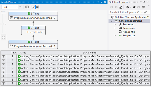
The whole work gets divided into two worker threads/tasks as shown in Figure 1:

Figure 1 - The Parallel Stacks window in Visual Studio 2010 ( #2 cores )

You can see that each thread is responsible for a range of values (data is partitioned among available cores). Thread 1 is evaluating the value 32983 and Thread 3 is evaluating 33073. This all occurs synchronously.

If I had a computer with 4 cores, the work would be divided into 4 threads/tasks and so on. If the time kept decreasing I’d achieve 1.5 seconds to run the app. Fantastic, isn’t it?

The new Microsoft Visual Studio 2010 (currently in Beta 2) comes with great debugging tooling for parallel applications as for example the Parallel Stacks shown in Figure 1 and the Parallel Tasks window shown in Figure 2:

Figure 2 - The Parallel Tasks window in Visual Studio 2010 ( #2 cores )

This post gives you a rapid view of PLINQ and how it can leverage the power of you current and future hardware.

The future as foreseen by hardware industry specialists is a multicore future. So why not get ready to it right now? You certainly can with PLINQ. It abstracts all the low level code to get parallel and let’s you focus on what’s important: your business domain.

If you want to go deep using PLINQ, I advise you to read Patterns for Parallel Programming: Understanding and Applying Parallel Patterns with the .NET Framework 4 by Stephen Toub.

Updated on February 15, 2013

Running this same sample app on a Intel Core i7-3720QM 2.6GHz quad-core processor (with #4 cores and #8 threads) this is the result:

Time elapsed: 00:00:00.8143775

This is on a par with the #1 core and #2 cores tests shown above. The work is being divided "almost" evenly by 8 if we compare with the first benchmark ( only #1 core ).

00:00:06.0252929 / 8 = 0.7525

Of course there’s been lots of improvements between these different processor generations. The software algorithms used to parallelize the work have also been improved (now I’m running on Visual Studio 2012 with .NET 4.5). Both hardware/software specs are higher now. Nonetheless these numbers give a good insight about the performance gains both in terms of hardware and software. Software developers like me have many reasons to celebrate!

Figure 3 - The Parallel Stacks window in Visual Studio 2012 ( #8 threads )

If I take out the .AsParallel() operator, the program runs on a single core and the time increases substantially:

Time elapsed: 00:00:03.4362160

If compared with the #4 cores benchmark above, we have:

00:00:03.4362160 / 4 = 0.8575

0.8575 – 0.8143 = 0.0432 (no difference at all)

Note: this faster processor running on a single core has a performance equivalent to the old Intel #2 core processor. Pretty interesting.

References
Features new to parallel debugging in VS 2010
Debugging Task-Based Parallel Applications in Visual Studio 2010 by Daniel Moth and Stephen Toub

Great lecture on what to expect from the multicore and parallel future…
Slides from Parallelism Tour by Stephen Toub

PLINQ documentation on MSDN
http://msdn.microsoft.com/en-us/library/dd460688%28VS.100%29.aspx

Parallel Computing Center on MSDN
http://msdn.microsoft.com/en-us/concurrency/default.aspx

Daniel Moth’s blog
http://www.danielmoth.com/Blog/index.htm

Microsoft Visual Studio 2010
http://www.microsoft.com/visualstudio/en-us/products/2010/default.mspx

Let’s say you have a list of integer values that represent the days of a month like this:

6, 2, 4, 1, 9, 7, 3, 10, 15, 19, 11, 18, 13, 22, 24, 20, 27, 31, 25, 28

Clearly we have missing numbers/days in the list above. They are:

5 8 12 14 16 17 21 23 26 29 30

It’s really easy to get a list of missing numbers using LINQ with C# and the Except operator. LINQ is the greatest addition to the C# language. I can imagine how life would be difficult if we hadn’t LINQ!

This is how I implemented a missing numbers finder using a C# extension method:

public static class MyExtensions
{
    /// <summary>
    /// Finds the missing numbers in a list.
    /// </summary>
    /// <param name="list">List of numbers</param>
    /// <returns>Missing numbers</returns>
    public static IEnumerable<int> FindMissing(this List<int> list)
    {
        // Sorting the list
        list.Sort();

        // First number of the list
        var firstNumber = list.First();

        // Last number of the list
        var lastNumber = list.Last();

        // Range that contains all numbers in the interval
        // [ firstNumber, lastNumber ]
        var range = Enumerable.Range(firstNumber, lastNumber - firstNumber);

        // Getting the set difference
        var missingNumbers = range.Except(list);

        return missingNumbers;
    }
}

Now you can call the extension method in the following way:

class Program
{
    static void Main(string[] args)
    {
        // List of numbers
        List<int> daysOfMonth =
            new List<int>() { 6, 2, 4, 1, 9, 7, 3, 10, 15, 19, 11, 18, 13, 22, 24, 20, 27, 31, 25, 28 };

        Console.Write("\nList of days: ");

        foreach(var num in daysOfMonth)
        {
            Console.Write("{0} ", num);
        }

        Console.Write("\n\nMissing days are: ");

        // Calling the Extension Method in the List of type int 
        foreach(var number in daysOfMonth.FindMissing())
        {
            Console.Write("{0} ", number);
        }
    }
}

This is the output:

 

In this simple program I’m using 3 concepts of the C# language that are really interesting: implicitly typed local variables, extension methods and collection initializers.

Hope this simple extension method to find the missing elements of a sequence helps the developers out there.

Visual Studio 2008 C# Console Application
You can get the Microsoft Visual Studio Project at:

http://leniel.googlepages.com/MissingNumbersFinder.zip

To try out the code you can use the free Microsoft Visual C# 2008 Express Edition that you can get at: http://www.microsoft.com/express/vcsharp/

A reader of the blog called Zip wrote a comment on the post Creating Excel spreadsheets .XLS and .XLSX in C#.

This is an excerpt from Zip’s comment:

… if I add rows using NPOI in C#, rows added under the table won't be automatically included in the table, and my chart is not updated the way I would like it to be.
How can I work around this problem?

I tried to simulate the problem with a simple spreadsheet and I was getting the same problem stated by Zip, that is, if I added one row just beneath the last row in the table, such added row wasn’t included in Excel’s data table and consequently the chart bound to the table wasn’t updated to reflect the new data.

To workaround this problem, let’s consider the following spreadsheet shown in Figure 1:

 
Figure 1 - NPOI with Excel Table and dynamic Chart

As you see we have a simple Excel data table with a players column that represents the name arguments of the chart, 4 columns for the months that form the category labels arguments (X axis) and the values arguments for the months going from Jan through Apr (Y axis).

Using NPOI to insert a new row in the table shown above we do the following:

// Creating a new row... 0 is the first row for NPOI.
HSSFRow row = sheet.CreateRow(5); // Row 6 in Excel

// Creating new cells in the row... 0 is the first column for NPOI.
row.CreateCell(1).SetCellValue("Eve Paradise"); // Column B
row.CreateCell(2).SetCellValue(4); // Column C
row.CreateCell(3).SetCellValue(3); // Column D
row.CreateCell(4).SetCellValue(2); // Column E
row.CreateCell(5).SetCellValue(1); // Column F 

The result is shown in Figure 2:

Figure 2 - NPOI with Excel Table and dynamic Chart - Adding a new row

Figure 2 shows us the problem stated by Zip in his comment. The new row we just added wasn’t included in the table. The chart that is linked to the table won’t update because it isn’t aware of the new row.

How to workaround this problem? That’s the question!

After playing with this case for 4 hours I’ve found a way of doing what Zip asks for.

Here’s how I did it:

Expand your Excel data table to row 10. I expanded only 4 rows just to show you how to workaround NPOI’s current limitation.

To expand your table, click in the minuscule handle in the lower-right corner of the cell occupying the lower-right corner of the table. This handle gives you a way to expand the table. Usually, it’s easier just to add data and let Excel expand the table - what doesn’t work with NPOI. But if you want to add several new rows or columns all at once, the handle is a good way to do it.

After expanding your table save the spreadsheet. It’ll be the template spreadsheet used to create new spreadsheets.

Figure 3 shows how the above spreadsheet looks like when the table is expanded to row 10:

Figure 3 - NPOI with Excel Table and dynamic Chart - Expanding the Table

We can see that row 6 added using NPOI is now part of the table because we expanded the table. The chart now shows the new data but we got a new problem: the chart shows empty (blank series) that are the reflection of the the empty rows we have on the data table - take a look at the chart’s legend for example and you’ll see squares that represent nothing.

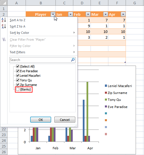
How to get over this? Well, we just need to filter the data in the table as shown in

Figure 4:

Figure 4 - NPOI with Excel Table and dynamic Chart - Filtering Data (blank series)

Filter out players removing the blank rows by unchecking (Blanks) circled in red in Figure 4. Doing so the chart will reflect the change showing only the filtered data as you see in Figure 5:

Figure 5 - NPOI with Excel Table and dynamic Chart - Filtered Data (no empty rows)

Now we have an Excel data table that is filtered (take a look at the funnel symbol) in the Player column. Other difference is that the rows that contain data are marked in blue. Although we have only 4 rows of data being displayed, our table has indeed 8 rows of data because we expanded it. The other 4 rows are hidden because they were filtered for not having any data yet.

Positioning the mouse cursor within the Excel data table, I’ll add a Total Row (option circled in red) in the table so that I can summarize data the way I want for each column as shown in Figure 6:

Figure 6 - NPOI with Excel Table and dynamic Chart - Adding Total Row

With this Excel template spreadsheet we can now use NPOI to fill our sheet with more 4 rows of data. Let’s do it. This is the code I used:

HSSFRow row7 = sheet.CreateRow(6);

row7.CreateCell(1).SetCellValue("David Goliath");
row7.CreateCell(2).SetCellValue(7);
row7.CreateCell(3).SetCellValue(7);
row7.CreateCell(4).SetCellValue(7);
row7.CreateCell(5).SetCellValue(7);

HSSFRow row8 = sheet.CreateRow(7);

row8.CreateCell(2).SetCellValue("Moses of Egypt");
row8.CreateCell(3).SetCellValue(8);
row8.CreateCell(4).SetCellValue(8);
row8.CreateCell(5).SetCellValue(8);
row8.CreateCell(6).SetCellValue(8);

HSSFRow row9 = sheet.CreateRow(8);

row9.CreateCell(1).SetCellValue("David Shepherd");
row9.CreateCell(2).SetCellValue(9);
row9.CreateCell(3).SetCellValue(9);
row9.CreateCell(4).SetCellValue(9);
row9.CreateCell(5).SetCellValue(9);

HSSFRow row10 = sheet.CreateRow(9);

row10.CreateCell(2).SetCellValue("Jesus of Nazareth");
row10.CreateCell(3).SetCellValue(10);
row10.CreateCell(4).SetCellValue(10);
row10.CreateCell(5).SetCellValue(10);
row10.CreateCell(6).SetCellValue(10);

// Forcing formula recalculation so that the Total Row gets updated
sheet.ForceFormulaRecalculation = true;

After filling the spreadsheet we get the result shown in Figure 7:

Figure 7 - NPOI with Excel Table and dynamic Chart - Chart updated automatically/dynamically

This is the workaround! :o)

The rows added with NPOI now are part of the table and are shown in the chart.

As a last hint: remember to expand your Excel data table to the number of rows you think your spreadsheet will store so that the rows added with NPOI get included in the table and the chart gets updated.

Again this is a good proof of what free software as is the case of NPOI can make for us. Even when dealing with more elaborated concepts as is the case of Excel tables and charts NPOI makes it easy to get the job done.

I wish that the next version of NPOI does what Zip wants automatically, that is, recognize rows added under the last row of an Excel table. At least we could have a parameter to let the user define if s/he wants the row to make part of the table or not.

Hope you enjoy this post.

Visual Studio 2008 C# ASP.NET MVC Web Application
You can get the Microsoft Visual Studio Project at:

http://leniel.googlepages.com/NPOIExcelTableChartMvcProject.zip

To try out the code you can use the free Microsoft Visual Web Developer 2008 Express Edition that you can get at: http://www.microsoft.com/express/vwd/Default.aspx